Fitting a Line to Data

The Getting started tutorial shows how to sample a 3D gaussian with simpple. In this tutorial, we will build on this to demonstrate a more realistic scenario where we fit a line to data.

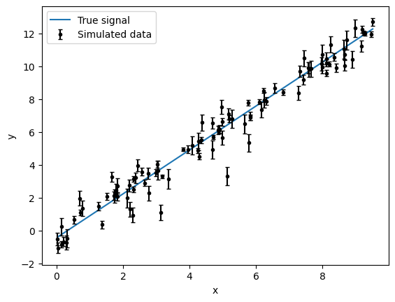
Simulated data

import matplotlib.pyplot as plt
import numpy as np

rng = np.random.default_rng(123)

x = np.sort(10 * rng.random(100))
m_true = 1.338
b_true = -0.45
truths = {"m": m_true, "b": b_true, "sigma": None}
y_true = m_true * x + b_true
yerr = 0.1 + 0.5 * rng.random(x.size)
y = y_true + 2 * yerr * rng.normal(size=x.size)

ax = plt.gca()
ax.plot(x, y_true, label="True signal")
ax.errorbar(x, y, yerr=yerr, fmt="k.", capsize=2, label="Simulated data")
ax.set_ylabel("y")
ax.set_xlabel("x")
plt.legend()
plt.show()

Linear model

To define our linear model with simpple, we could directly write the log-likelihood function and calculate the model inside of it. A slightly more granular approach is to first define our “forward model” function and then call that function from the log-likelihood. Notice that we add an extra parameter to inflate the uncertainties in the likelihood.

def linear_model(p, x):
    return p["m"] * x + p["b"]


def log_likelihood(p, x, y, yerr):
    ymod = linear_model(p, x)
    var = yerr**2 + p["sigma"] ** 2
    return -0.5 * np.sum(np.log(2 * np.pi * var) + (y - ymod) ** 2 / var)

simpple has a dedicated class for models that consist of a forward model called in the likelihood: simpple.model.ForwardModel. Using this class instead of the base Model has two main advantages: we can sample predictions from the prior with get_prior_pred() and the forward model, accessible through ForwardModel.forward() is wrapped to accept either a dictionary or an array.

Let us define our linear model. We will use uniform priors on the linear parameters and a log-uniform on sigma.

from simpple.distributions import Uniform, LogUniform

from simpple.model import ForwardModel

parameters = {
    "m": Uniform(-10, 10),
    "b": Uniform(-10, 10),
    "sigma": LogUniform(1e-5, 100),
}

model = ForwardModel(parameters, log_likelihood, linear_model)

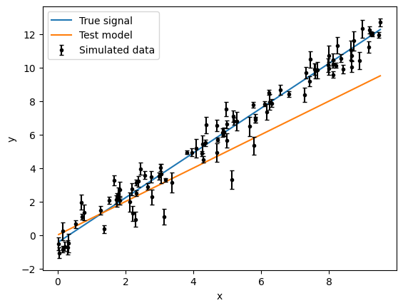
First, we can check that the model works as expected on a single test point. Note that all arguments required by the likelihood are also required by the log-posterior (log_prob()) They will then be passed to the likelihood internally.

test_point = {"m": 1.0, "b": 0, "sigma": 1.0}
print(model)
print("Log prior", model.log_prior(test_point))
print("Log likelihood", model.log_likelihood(test_point, x, y, yerr))
print("Log probability", model.log_prob(test_point, x, y, yerr))

ForwardModel(parameters={'m': Uniform(low=-10, high=10), 'b': Uniform(low=-10, high=10), 'sigma': LogUniform(low=1e-05, high=100)}, log_likelihood=log_likelihood, forward=linear_model)
Log prior -8.77140714141125
Log likelihood -212.35014668988225
Log probability -221.1215538312935

ax = plt.gca()
ax.plot(x, y_true, label="True signal")
ax.plot(x, model.forward(test_point, x), label="Test model")
ax.errorbar(x, y, yerr=yerr, fmt="k.", capsize=2, label="Simulated data")
ax.set_ylabel("y")
ax.set_xlabel("x")
plt.legend()
plt.show()

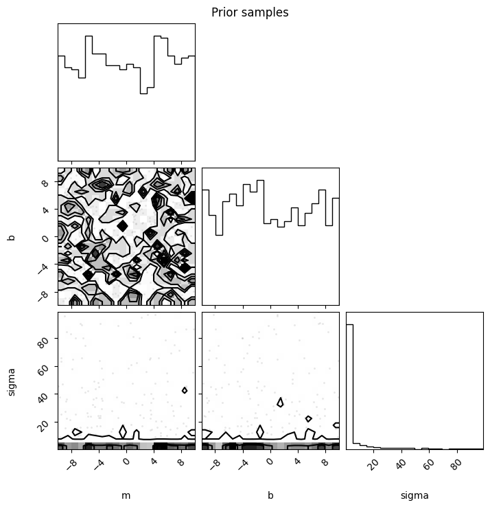
Prior checks

First, we can do a prior check. We will look at the joint prior on parameters to make sure that we did not make any mistake in our specification.

Note: We use corner to display the posterior. You will need to install it along with arviz to display the prior and posterior distributions.

import corner

n_prior = 1000
prior_samples = model.get_prior_samples(n_prior)

fig = corner.corner(prior_samples)
fig.suptitle("Prior samples")
plt.show()

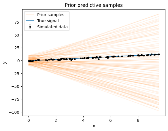
We can also look at forward model predictions for prior samples. This gives a good idea of whether the parameter space covers all the data and yields reasonable models.

n_pred = 100
ypreds = model.get_prior_pred(n_pred, x)
ax = plt.gca()
for i, ypred in enumerate(ypreds):
    ax.plot(x, ypred, "C1-", label="Prior samples" if i == 0 else None, alpha=0.1)
ax.plot(x, y_true, label="True signal")
ax.errorbar(x, y, yerr=yerr, fmt="k.", capsize=2, label="Simulated data")
ax.set_ylabel("y")
ax.set_xlabel("x")
ax.set_title("Prior predictive samples")
plt.legend()
plt.show()

Posterior sampling

To sample the posterior distribution, let us use the zeus-mcmc package. Feel free to replace this with your favorite MCMC or nested sampling library.

import zeus

nwalkers = 100
nsteps = 1000
ndim = len(model.keys())
start = np.array([0.0, 0.0, 10.0]) + rng.standard_normal(size=(nwalkers, ndim))
sampler = zeus.EnsembleSampler(nwalkers, ndim, model.log_prob, args=(x, y, yerr))
sampler.run_mcmc(start, nsteps, progress=False)

Initialising ensemble of 100 walkers...

/home/docs/checkouts/readthedocs.org/user_builds/simpple/envs/stable/lib/python3.12/site-packages/simpple/distributions.py:423: RuntimeWarning: invalid value encountered in log
  -np.log(x * np.log(self.high / self.low)),

Posterior distribution and predictions

Just like we did for the prior, we can now visualize the posterior and some predictive samples drawn from the posterior.

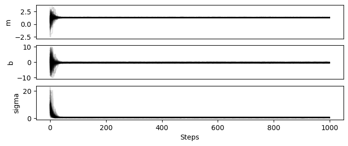
First, let us look at the chains to make sure they are well-behaved. It is quite common to show the chains in plot like the one below, and they are somewhat cumbersome to code. For that reason, simpple comes with a chainplot utility function.

from simpple.plot import chainplot

chains = sampler.get_chain()
chainplot(chains, labels=model.keys())
plt.show()

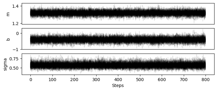
200 seems like a safe warm-up in this case!

chains = sampler.get_chain(discard=200)
chainplot(chains, labels=model.keys())
plt.show()

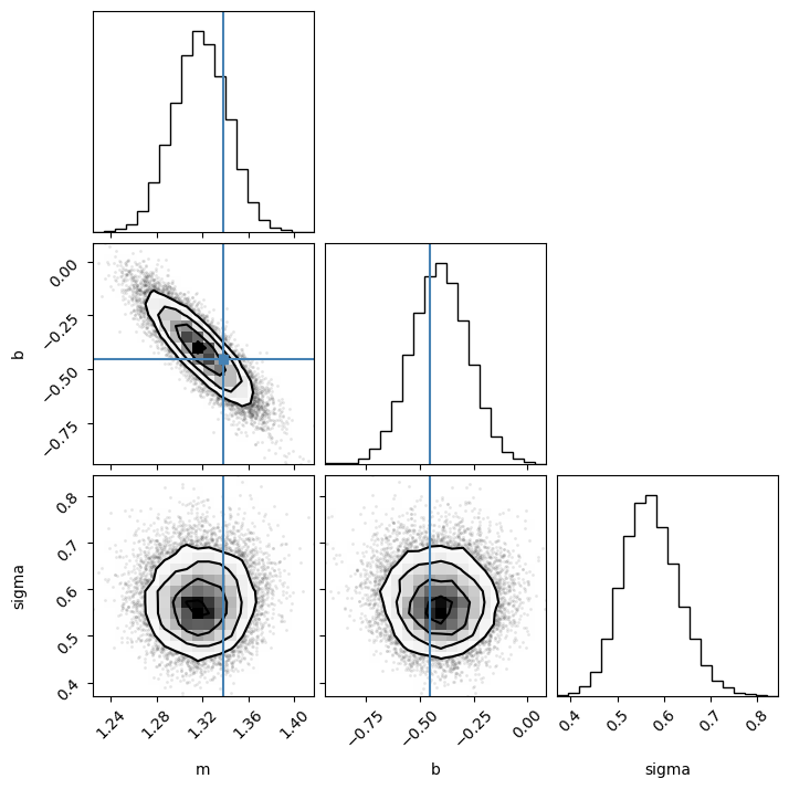
flat_chains = sampler.get_chain(discard=200, flat=True, thin=5)
corner.corner(
    flat_chains,
    labels=model.keys(),
    truths=list(truths.values()),
)
plt.show()

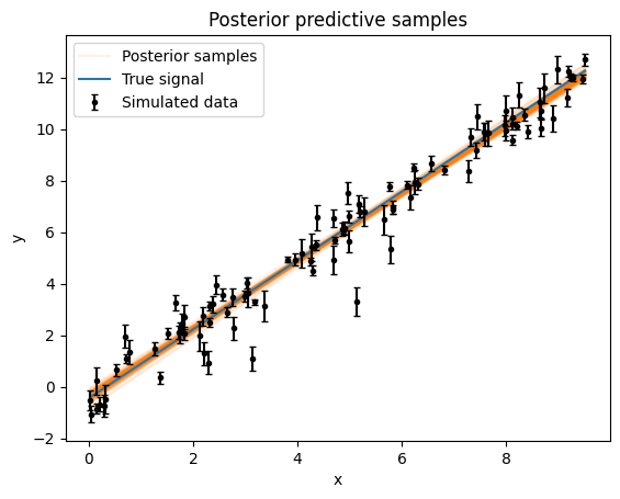
To sample posterior predictions of the forward model, we need to use the get_posterior_pred() function. It takes both the chains and a number of samples for arguments. n_pred samples will be drawn from the chain at random.

n_pred = 100
ypreds = model.get_posterior_pred(flat_chains.T, n_pred, x)
ax = plt.gca()
for i, ypred in enumerate(ypreds):
    ax.plot(x, ypred, "C1-", label="Posterior samples" if i == 0 else None, alpha=0.1)
ax.plot(x, y_true, label="True signal")
ax.errorbar(x, y, yerr=yerr, fmt="k.", capsize=2, label="Simulated data")
ax.set_ylabel("y")
ax.set_xlabel("x")
ax.set_title("Posterior predictive samples")
plt.legend()
plt.show()

This notebook shows all the basic steps to perform Bayesian inference with simpple. The main things that will change in real usage are the forward model and prior definitions (and of course the data). Everything else from this notebook should be re-usable almost as-is.