Getting started#
The goal of simpple is to have a tiny probablistic programming language compatible with some of the most common sampling libraries.
That way, it is easy to write a model (including all priors) for emcee, and then run it with nautilus, for example.
In this tutorial, we will do a short demo by sampling a 3D normal distribution.
import simpple

print(simpple.__version__)
0.3.4
Model Definition#
The two key components we need to specify in a Bayesian model are the prior distribution and the likelihood function. Pretty much all sampling libraries require these two components, either separately for nested sampling, or combined in a posterior for MCMC.
In simpple, the prior is specified as a dictionary of Distribution objects.
Most common distributions are already implemented in scipy, but they are much slower than custom implementations. The recommended approach is therefore to use simpple’s distributions whenever possible.
Note
If the distribution you want is not available, you can either implement it yourself (see the source code for examples) or open an issue on GitHub.
from simpple.distributions import Uniform, Normal

parameters = {
    "x1": Uniform(-5, 5),
    "x2": Uniform(0, 10),
    "x3": Normal(0, 10),
}
print("Priors:")
print(parameters)
Priors:
{'x1': Uniform(low=-5, high=5), 'x2': Uniform(low=0, high=10), 'x3': Normal(mu=0, sigma=10)}
Next, we need a log-likelihood function that takes a dictionary of parameters and computes the likelihood.
In this simple 3D Gaussian example, we compare each parameter directly with a “data point” (mean), and the noise is correlated (defined by cov).
Here we use scipy for convenience, but again in real-world scenarios custom implementations will be faster.
from scipy.stats import multivariate_normal


def log_likelihood(params):
    """Log-likelihood function for a 3D normal distribution."""
    p = [params["x1"], params["x2"], params["x3"]]
    mean = [0.0, 3.0, 2.0]
    cov = [[1, 0.5, 0], [0.5, 1, 0], [0, 0, 1.0]]
    return multivariate_normal.logpdf(p, mean=mean, cov=cov)
It is now time to create our simpple.Model object.
The model needs to know what our priors and likelihood are.
It will then wrap them to provide:
Model.log_prior(parameters): the prior distribution given a dictionary or an array of parametersModel.log_prob(parameters): the posterior distribution given a dictionary or an array of parametersModel.log_likelihood(parameters): a wrapper around our log-likelihood above to make it work with arrays and dictionariesModel.prior_transform(u): a prior transform from a unit hypercube to our parameter space
from simpple.model import Model

model = Model(parameters, log_likelihood)

print(model)
test_point = [0, 1, 0]
print("Log-Prior", model.log_prior(test_point))
print("Log-Prior out of bounds", model.log_prior([-10, 3, 0]))
print("Log-likelihood", model.log_likelihood(test_point))
print("Log-posterior", model.log_prob(test_point))
Model(parameters={'x1': Uniform(low=-5, high=5), 'x2': Uniform(low=0, high=10), 'x3': Normal(mu=0, sigma=10)}, log_likelihood=log_likelihood)
Log-Prior -7.826693812186811
Log-Prior out of bounds -inf
Log-likelihood -7.279641230054793
Log-posterior -15.106335042241604
Prior Checks#
A good thing to do before fitting any model is to check the prior.
To sample directly from the prior, we can either pass a uniform distribution through the prior_transform function or sample the log_prior() function of our model with emcee.
Here, we will test both approaches. In practice, it’s probably a good idea to test your prior transform if you plan on using nested sampling and your log-prior if you plan on using MCMC.
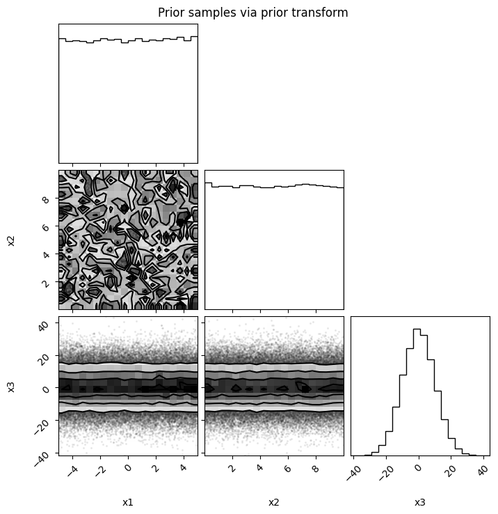
Via prior transform#
import corner
import matplotlib.pyplot as plt
import numpy as np

rng = np.random.default_rng()
u = np.random.uniform(0, 1, size=(3, 100_000))
prior_samples = model.prior_transform(u)

fig = corner.corner(prior_samples.T, labels=model.keys())
fig.suptitle("Prior samples via prior transform")
plt.show()
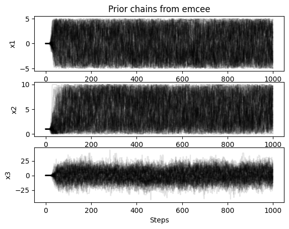
Via emcee#
import emcee

sampler = emcee.EnsembleSampler(
    nwalkers=100,
    ndim=3,
    log_prob_fn=model.log_prior,
)
p0 = np.array(test_point) + 1e-4 * rng.standard_normal(size=(100, 3))
_ = sampler.run_mcmc(p0, 1000, progress=True)
0%| | 0/1000 [00:00<?, ?it/s]
5%|▌ | 52/1000 [00:00<00:01, 518.92it/s]
10%|█ | 104/1000 [00:00<00:01, 519.04it/s]
16%|█▌ | 157/1000 [00:00<00:01, 520.60it/s]
21%|██ | 210/1000 [00:00<00:01, 521.77it/s]
26%|██▋ | 263/1000 [00:00<00:01, 521.97it/s]
32%|███▏ | 316/1000 [00:00<00:01, 522.22it/s]
37%|███▋ | 369/1000 [00:00<00:01, 522.25it/s]
42%|████▏ | 422/1000 [00:00<00:01, 521.76it/s]
48%|████▊ | 475/1000 [00:00<00:01, 521.32it/s]
53%|█████▎ | 528/1000 [00:01<00:00, 521.30it/s]
58%|█████▊ | 581/1000 [00:01<00:00, 520.88it/s]
63%|██████▎ | 634/1000 [00:01<00:00, 521.56it/s]
69%|██████▊ | 687/1000 [00:01<00:00, 521.81it/s]
74%|███████▍ | 740/1000 [00:01<00:00, 521.72it/s]
79%|███████▉ | 793/1000 [00:01<00:00, 522.22it/s]
85%|████████▍ | 846/1000 [00:01<00:00, 521.48it/s]
90%|████████▉ | 899/1000 [00:01<00:00, 521.96it/s]
95%|█████████▌| 952/1000 [00:01<00:00, 521.83it/s]
100%|██████████| 1000/1000 [00:01<00:00, 521.59it/s]
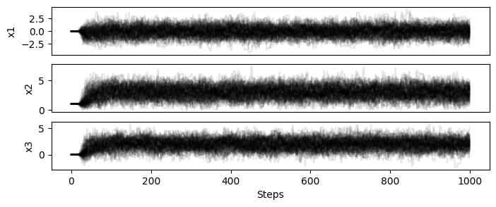
chains = sampler.get_chain()

fig, axs = plt.subplots(3, 1)
for i in range(3):
    axs[i].plot(chains[:, :, i], "k-", alpha=0.1)
    axs[i].set_ylabel(model.keys()[i])
axs[-1].set_xlabel("Steps")
axs[0].set_title("Prior chains from emcee")
plt.show()
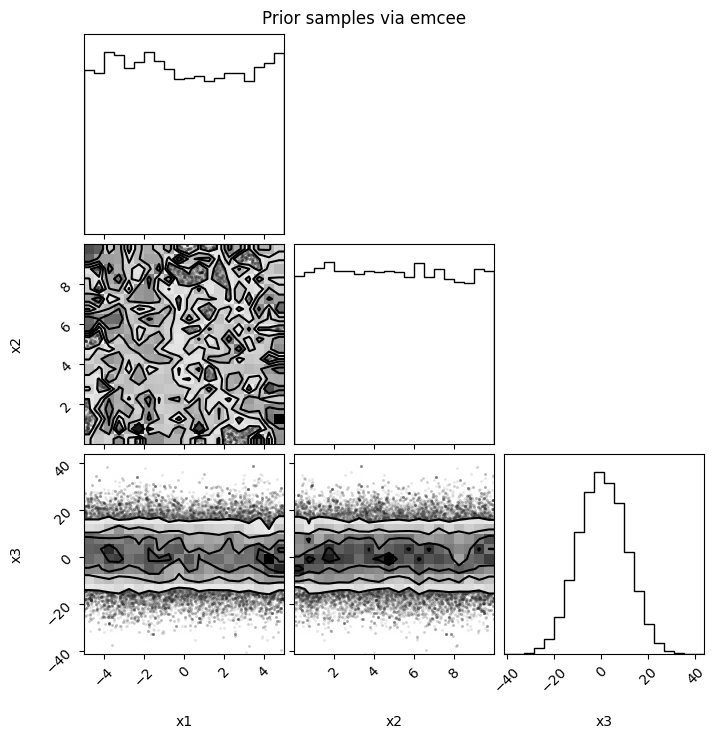
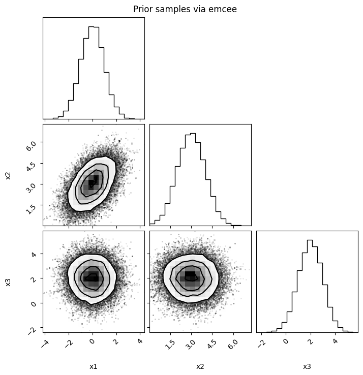
flat_chains = sampler.get_chain(discard=200, flat=True)
fig = corner.corner(flat_chains, labels=model.keys())
fig.suptitle("Prior samples via emcee")
plt.show()
Sampling the Posterior with emcee#
We can now sample the posterior with emcee!
sampler = emcee.EnsembleSampler(
    nwalkers=100,
    ndim=model.ndim,
    log_prob_fn=model.log_prob,
)
p0 = np.array(test_point) + 1e-4 * rng.standard_normal(size=(100, model.ndim))
_ = sampler.run_mcmc(p0, 1000, progress=True)
0%| | 0/1000 [00:00<?, ?it/s]
1%| | 11/1000 [00:00<00:09, 102.97it/s]
2%|▏ | 22/1000 [00:00<00:09, 103.47it/s]
3%|▎ | 33/1000 [00:00<00:09, 104.33it/s]
4%|▍ | 44/1000 [00:00<00:09, 105.30it/s]
6%|▌ | 55/1000 [00:00<00:08, 106.00it/s]
7%|▋ | 66/1000 [00:00<00:08, 106.20it/s]
8%|▊ | 77/1000 [00:00<00:08, 106.72it/s]
9%|▉ | 88/1000 [00:00<00:08, 106.70it/s]
10%|▉ | 99/1000 [00:00<00:08, 106.62it/s]
11%|█ | 110/1000 [00:01<00:08, 106.25it/s]
12%|█▏ | 121/1000 [00:01<00:08, 105.65it/s]
13%|█▎ | 132/1000 [00:01<00:08, 105.68it/s]
14%|█▍ | 143/1000 [00:01<00:08, 105.60it/s]
15%|█▌ | 154/1000 [00:01<00:08, 105.59it/s]
16%|█▋ | 165/1000 [00:01<00:07, 105.69it/s]
18%|█▊ | 176/1000 [00:01<00:07, 105.92it/s]
19%|█▊ | 187/1000 [00:01<00:07, 106.04it/s]
20%|█▉ | 198/1000 [00:01<00:07, 105.76it/s]
21%|██ | 209/1000 [00:01<00:07, 105.66it/s]
22%|██▏ | 220/1000 [00:02<00:07, 106.16it/s]
23%|██▎ | 231/1000 [00:02<00:07, 106.37it/s]
24%|██▍ | 242/1000 [00:02<00:07, 106.14it/s]
25%|██▌ | 253/1000 [00:02<00:07, 106.00it/s]
26%|██▋ | 264/1000 [00:02<00:06, 105.72it/s]
28%|██▊ | 275/1000 [00:02<00:06, 105.86it/s]
29%|██▊ | 286/1000 [00:02<00:06, 105.79it/s]
30%|██▉ | 297/1000 [00:02<00:06, 105.64it/s]
31%|███ | 308/1000 [00:02<00:06, 105.77it/s]
32%|███▏ | 319/1000 [00:03<00:06, 105.71it/s]
33%|███▎ | 330/1000 [00:03<00:06, 105.52it/s]
34%|███▍ | 341/1000 [00:03<00:06, 105.85it/s]
35%|███▌ | 352/1000 [00:03<00:06, 106.14it/s]
36%|███▋ | 363/1000 [00:03<00:06, 106.00it/s]
37%|███▋ | 374/1000 [00:03<00:05, 105.98it/s]
38%|███▊ | 385/1000 [00:03<00:05, 105.75it/s]
40%|███▉ | 396/1000 [00:03<00:05, 105.71it/s]
41%|████ | 407/1000 [00:03<00:05, 105.76it/s]
42%|████▏ | 418/1000 [00:03<00:05, 105.72it/s]
43%|████▎ | 429/1000 [00:04<00:05, 105.68it/s]
44%|████▍ | 440/1000 [00:04<00:05, 105.88it/s]
45%|████▌ | 451/1000 [00:04<00:05, 106.01it/s]
46%|████▌ | 462/1000 [00:04<00:05, 105.58it/s]
47%|████▋ | 473/1000 [00:04<00:04, 105.54it/s]
48%|████▊ | 484/1000 [00:04<00:04, 105.85it/s]
50%|████▉ | 495/1000 [00:04<00:04, 105.34it/s]
51%|█████ | 506/1000 [00:04<00:04, 105.20it/s]
52%|█████▏ | 517/1000 [00:04<00:04, 105.05it/s]
53%|█████▎ | 528/1000 [00:04<00:04, 105.27it/s]
54%|█████▍ | 539/1000 [00:05<00:04, 105.38it/s]
55%|█████▌ | 550/1000 [00:05<00:04, 105.56it/s]
56%|█████▌ | 561/1000 [00:05<00:04, 105.60it/s]
57%|█████▋ | 572/1000 [00:05<00:04, 105.41it/s]
58%|█████▊ | 583/1000 [00:05<00:03, 105.63it/s]
59%|█████▉ | 594/1000 [00:05<00:03, 105.81it/s]
60%|██████ | 605/1000 [00:05<00:03, 105.85it/s]
62%|██████▏ | 616/1000 [00:05<00:03, 105.75it/s]
63%|██████▎ | 627/1000 [00:05<00:03, 105.57it/s]
64%|██████▍ | 638/1000 [00:06<00:03, 105.58it/s]
65%|██████▍ | 649/1000 [00:06<00:03, 105.81it/s]
66%|██████▌ | 660/1000 [00:06<00:03, 105.81it/s]
67%|██████▋ | 671/1000 [00:06<00:03, 106.07it/s]
68%|██████▊ | 682/1000 [00:06<00:03, 105.94it/s]
69%|██████▉ | 693/1000 [00:06<00:02, 105.60it/s]
70%|███████ | 704/1000 [00:06<00:02, 105.58it/s]
72%|███████▏ | 715/1000 [00:06<00:02, 105.73it/s]
73%|███████▎ | 726/1000 [00:06<00:02, 105.51it/s]
74%|███████▎ | 737/1000 [00:06<00:02, 105.38it/s]
75%|███████▍ | 748/1000 [00:07<00:02, 105.41it/s]
76%|███████▌ | 759/1000 [00:07<00:02, 105.92it/s]
77%|███████▋ | 770/1000 [00:07<00:02, 105.93it/s]
78%|███████▊ | 781/1000 [00:07<00:02, 105.57it/s]
79%|███████▉ | 792/1000 [00:07<00:01, 105.61it/s]
80%|████████ | 803/1000 [00:07<00:01, 105.56it/s]
81%|████████▏ | 814/1000 [00:07<00:01, 105.91it/s]
82%|████████▎ | 825/1000 [00:07<00:01, 105.64it/s]
84%|████████▎ | 836/1000 [00:07<00:01, 105.62it/s]
85%|████████▍ | 847/1000 [00:08<00:01, 105.74it/s]
86%|████████▌ | 858/1000 [00:08<00:01, 105.56it/s]
87%|████████▋ | 869/1000 [00:08<00:01, 105.43it/s]
88%|████████▊ | 880/1000 [00:08<00:01, 105.53it/s]
89%|████████▉ | 891/1000 [00:08<00:01, 105.50it/s]
90%|█████████ | 902/1000 [00:08<00:00, 105.75it/s]
91%|█████████▏| 913/1000 [00:08<00:00, 105.83it/s]
92%|█████████▏| 924/1000 [00:08<00:00, 105.74it/s]
94%|█████████▎| 935/1000 [00:08<00:00, 105.63it/s]
95%|█████████▍| 946/1000 [00:08<00:00, 105.59it/s]
96%|█████████▌| 957/1000 [00:09<00:00, 105.43it/s]
97%|█████████▋| 968/1000 [00:09<00:00, 105.69it/s]
98%|█████████▊| 979/1000 [00:09<00:00, 105.90it/s]
99%|█████████▉| 990/1000 [00:09<00:00, 106.03it/s]
100%|██████████| 1000/1000 [00:09<00:00, 105.71it/s]
from simpple.plot import chainplot

chains = sampler.get_chain()

chainplot(chains, labels=model.keys())
plt.show()
flat_chains = sampler.get_chain(discard=200, flat=True)
fig = corner.corner(flat_chains, labels=model.keys())
fig.suptitle("Prior samples via emcee")
plt.show()
Sampling with ultranest#
Next, let us try and sample the model with Ultranest.
import ultranest

sampler = ultranest.ReactiveNestedSampler(
    model.keys(), model.log_likelihood, model.prior_transform
)

result = sampler.run(show_status=False)
[ultranest] Sampling 400 live points from prior ...
[ultranest] Explored until L=-3
[ultranest] Likelihood function evaluations: 6088
[ultranest] logZ = -7.806 +- 0.08015
[ultranest] Effective samples strategy satisfied (ESS = 1862.9, need >400)
[ultranest] Posterior uncertainty strategy is satisfied (KL: 0.46+-0.05 nat, need <0.50 nat)
[ultranest] Evidency uncertainty strategy is satisfied (dlogz=0.08, need <0.5)
[ultranest] logZ error budget: single: 0.10 bs:0.08 tail:0.01 total:0.08 required:<0.50
[ultranest] done iterating.
sampler.print_results()
logZ = -7.786 +- 0.182
  single instance: logZ = -7.786 +- 0.096
  bootstrapped   : logZ = -7.806 +- 0.182
  tail           : logZ = +- 0.010
insert order U test : converged: True correlation: inf iterations

    x1                  : -3.72 │ ▁  ▁▁▁▁▂▂▂▃▅▅▆▆▇▇▇▇▇▇▇▅▄▃▃▂▂▁▁▁▁▁▁▁ ▁ │4.01      -0.00 +- 0.99
    x2                  : 0.00  │▁▁▁▁▁▁▂▂▃▃▄▅▆▆▇▇▇▆▆▆▆▅▄▄▃▃▂▁▁▁▁▁▁▁▁▁▁▁ │7.08      2.99 +- 0.99
    x3                  : -1.90 │ ▁▁▁▁▁▁▁▁▂▂▃▃▅▆▆▇▇▇▇▆▅▅▄▃▃▂▁▁▁▁▁▁▁   ▁ │6.44      1.98 +- 0.99
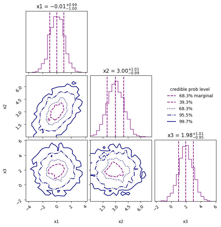
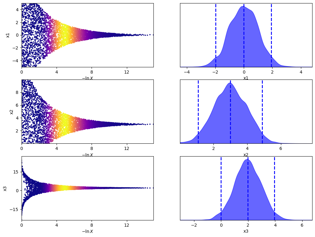
sampler.plot_corner()
plt.show()
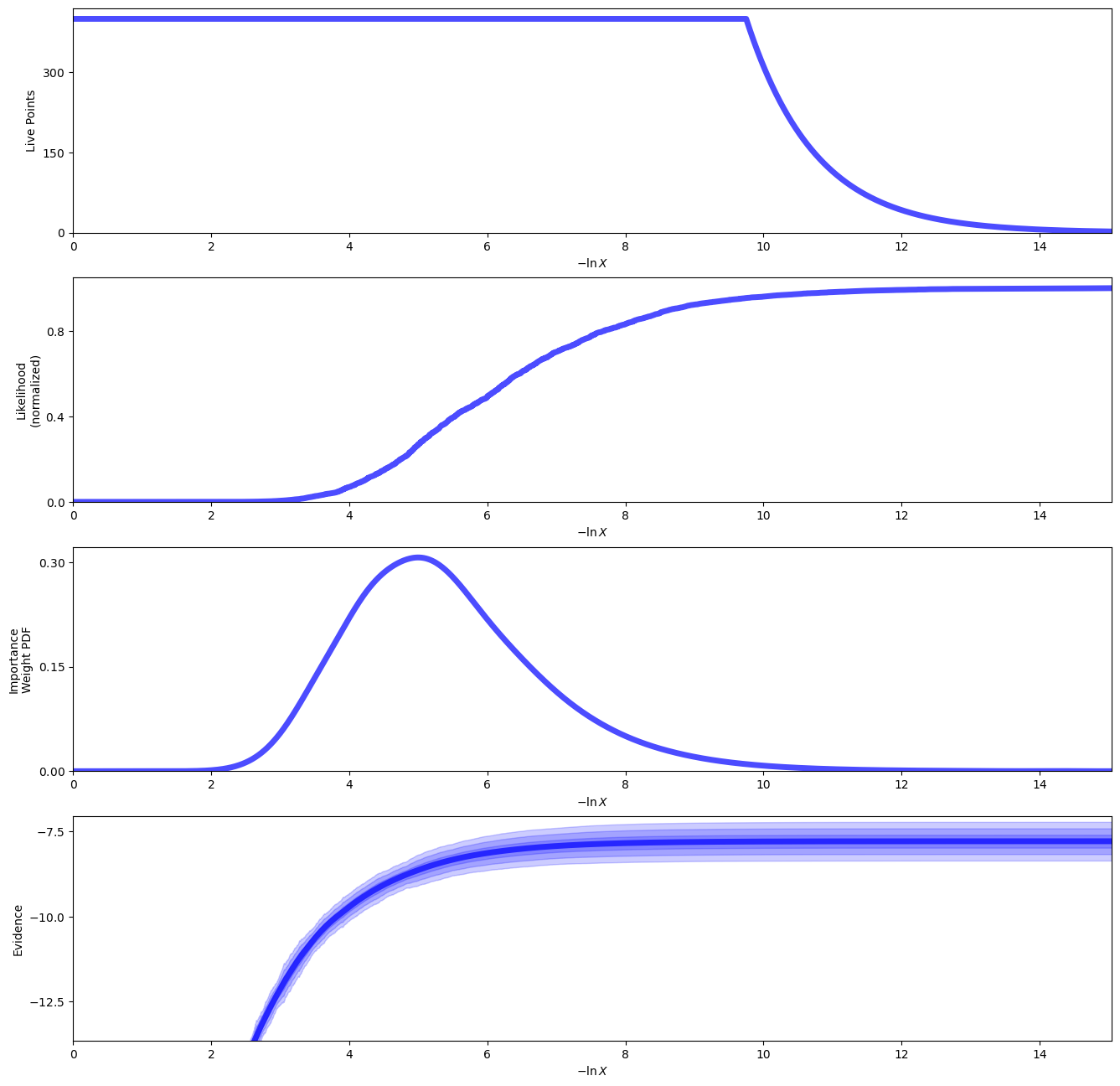
sampler.plot_run()
plt.show()
sampler.plot_trace()
plt.show()
Sampling with nautilus#
The Nautilus sampler uses a slightly different format for the prior specification.
simpple can also interface with nautilus using Model.nautilus_prior()!
from nautilus import Sampler

sampler = Sampler(model.nautilus_prior(), model.log_likelihood, n_live=1000)
sampler.run(verbose=False);
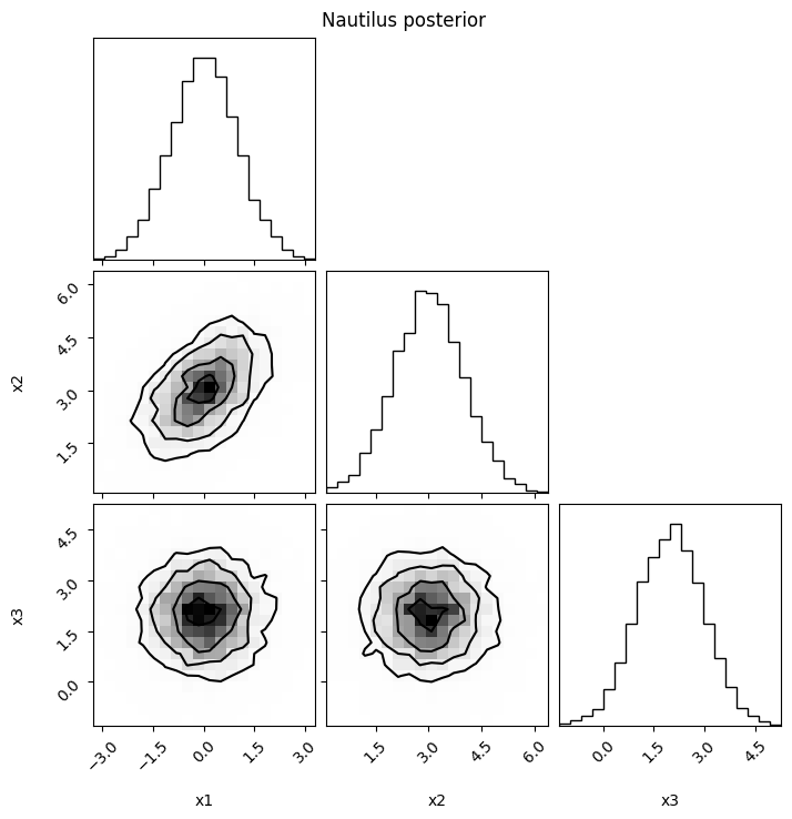
points, log_w, log_l = sampler.posterior()
fig = corner.corner(
    points,
    weights=np.exp(log_w),
    labels=model.keys(),
    plot_datapoints=False,
    range=np.repeat(0.999, len(model.parameters)),
)
fig.suptitle("Nautilus posterior")
plt.show()
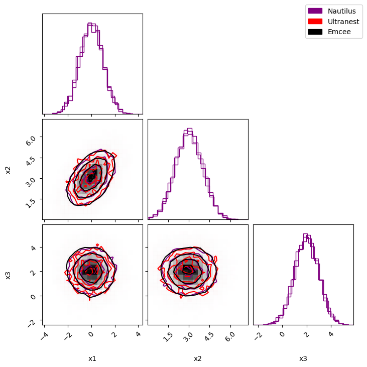
Comparison#
Now that we have explored the posterior with several samplers, we can compare the resulting distributions.
from matplotlib import patches

hist_kwargs = dict(density=True)

fig = corner.corner(
    points,
    weights=np.exp(log_w),
    labels=model.keys(),
    color="purple",
    hist_kwargs=hist_kwargs,
    plot_datapoints=False,
    range=np.repeat(0.999, len(model.parameters)),
)
data = np.array(result["weighted_samples"]["points"])
weights = np.array(result["weighted_samples"]["weights"])
corner.corner(
    data,
    weights=weights,
    color="red",
    hist_kwargs=hist_kwargs,
    plot_datapoints=False,
    range=np.repeat(0.999, len(model.parameters)),
    fig=fig,
)
corner.corner(
    flat_chains,
    weights=np.ones(flat_chains.shape[0]),
    color="k",
    hist_kwargs=hist_kwargs,
    plot_datapoints=False,
    fig=fig,
)


nautilus_patch = patches.Patch(color="purple", label="Nautilus")
ultranest_patch = patches.Patch(color="red", label="Ultranest")
emcee_patch = patches.Patch(color="k", label="Emcee")

fig.legend(
    handles=[nautilus_patch, ultranest_patch, emcee_patch],
    loc="upper right",  # You can also use 'upper left', 'lower right', etc.
    bbox_to_anchor=(0.98, 0.98),
)

plt.show()